***Please enjoy this blog posted on behalf of the author Kathy Dallaire, CEDS, eDiscovery and Litigation Support Coordinator, Stikeman Elliot LLP.
In this blog, we will demonstrate some handy Excel formulas commonly used to build load files where the information required is spread out over multiple spreadsheets or has been parsed out into separate cells.
While there can be numerous situations which require manually building a load file, hopefully these tips will save you some time and effort.
Combining values from multiple spreadsheets using VLookup.
In this scenario, we want to append values for Title and Filename from separate sheets of an Excel spreadsheet, to the Date value already in the first sheet, using the common DocID value.
The VLOOKUP formula uses the following arguments:
VLOOKUP(lookup_value, table_array, col_index_num, [range_lookup])
Lookup_value the identifier in all tables, for example the DocID. This value must be in the leftmost column of each table.
Table_array range where the value is to be retrieved either in another sheet of the same workbook or in another workbook altogether.
Col_index_num this is the column placement number in the range determined for Table_array where the matching value should be searched for.
Range_lookup TRUE to find the closest match or FALSE to find an exact match
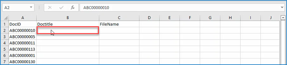
Click in the cell where the Doctitle value will be added:
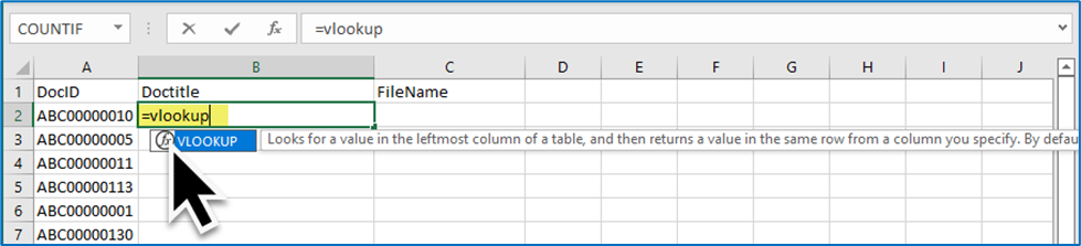
Start typing the formula =vlookup and click on the formula button :
The first argument is the lookup_value (or identifier in this case) – click on the cell with the value or type A2:
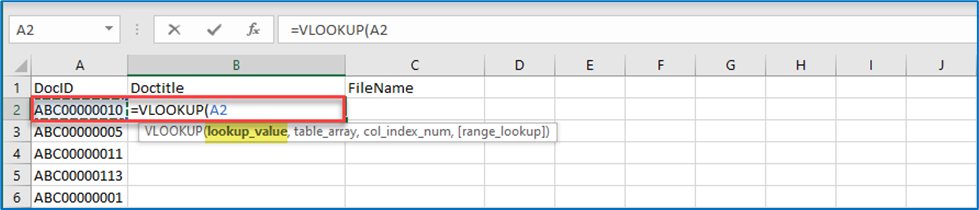
a. Add a comma after the cell number to enter the next argument,
table_array
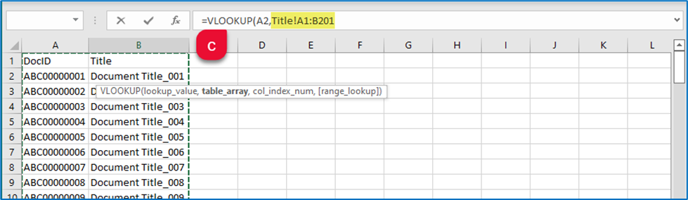
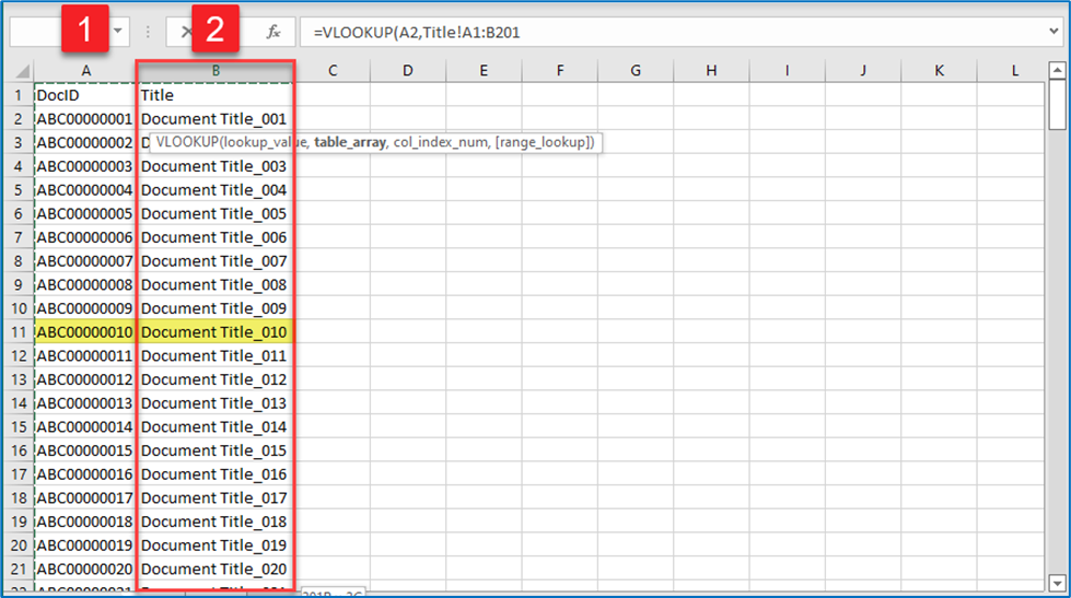
b. Open the sheet which contains the Doctitle values
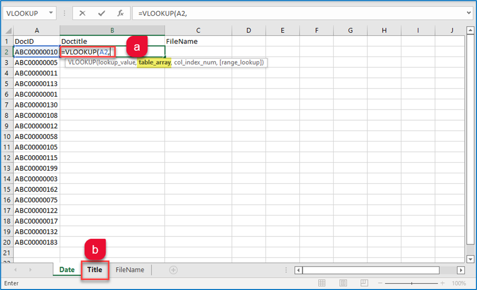
c. Select the range of data in which to search for the identified value (DocID). In this case the range is in the sheet named “Title” and in columns A and B between lines 1 and 201. Notice the range of selected cells is added to the formula:
Add a comma after to range to move to the next criteria, Col_index_num. This will be the number of the selected column in the selected range where the value is located (2):
Again, add a comma after the Col_index_num to continue to the final argument [range_lookup]. Select FALSE by double-clicking on it and close the parenthesis:
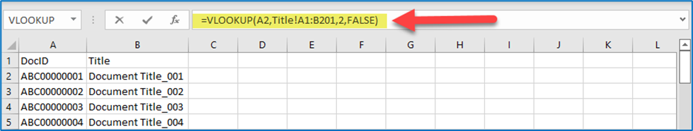
Press Enter to confirm the completed formula and the value will be added to the selected cell:
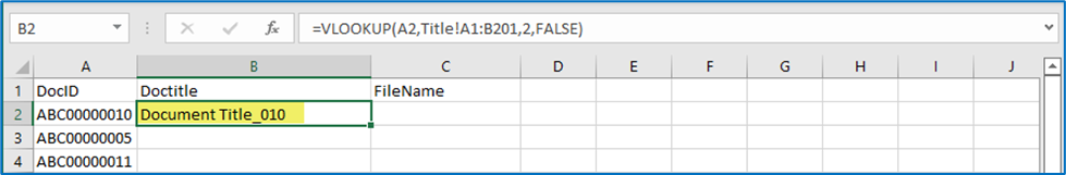
To auto complete the following lines, double-click or grab and drag the small fill handle down the column and they will auto complete:
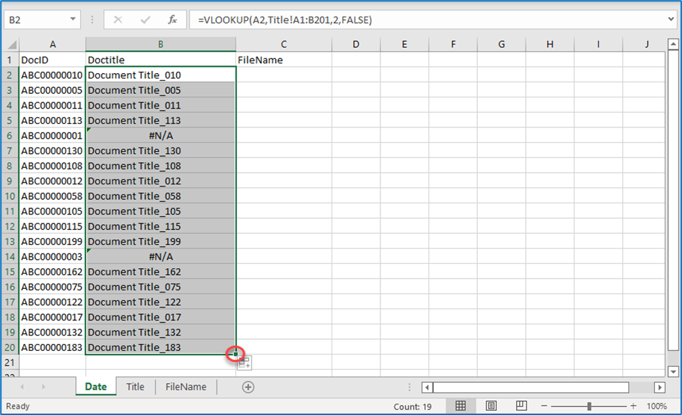
Notice that the value in two rows has failed to complete:
Notice that the value in two rows has failed to complete:
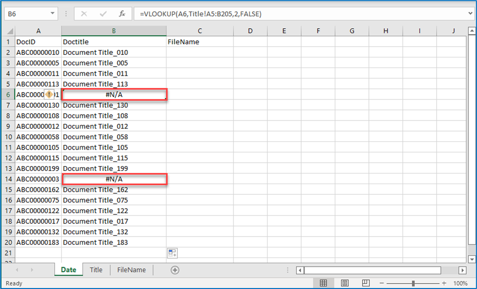
This is because as the relative formula is copied down the row and is updated with a new range each time it is copied down.
The initial formula in the first cell is:

and on row 6 it is:

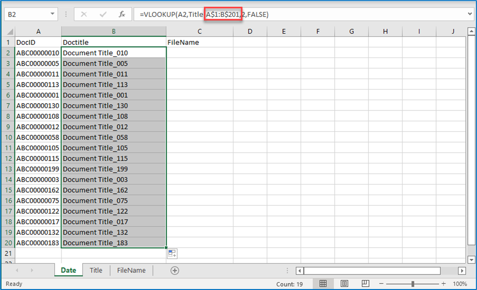
In order to copy the absolute formula down the row, modify the formula as follows in the first cell, before copying it down the row. Adding the $ symbol as indicated, will prevent the formula from updating as it is copied down:
Hard-Coding the Formula Results
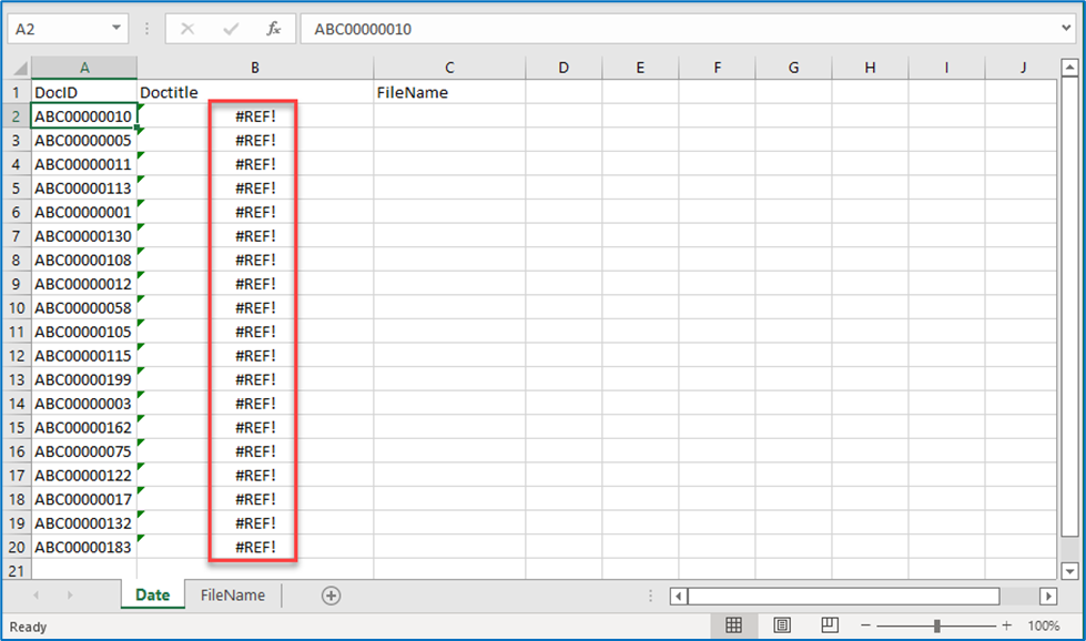
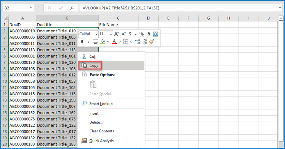
Finally, although when looking at the results, they appear to be correctly reflected, if you look in the formula bar, the contents is the formula and not the actual text. The values must be copy-pasted as text in order to be of any use. Furthermore, should the values in the range searched be modified, the changes would be reflected in the results of the formula. By the same token, should the sheet identified by the range in the formula be deleted from the spreadsheet or moved, the resulting value will be an error:
To prevent this, select and copy the row with the results of the VLOOKUP formula:
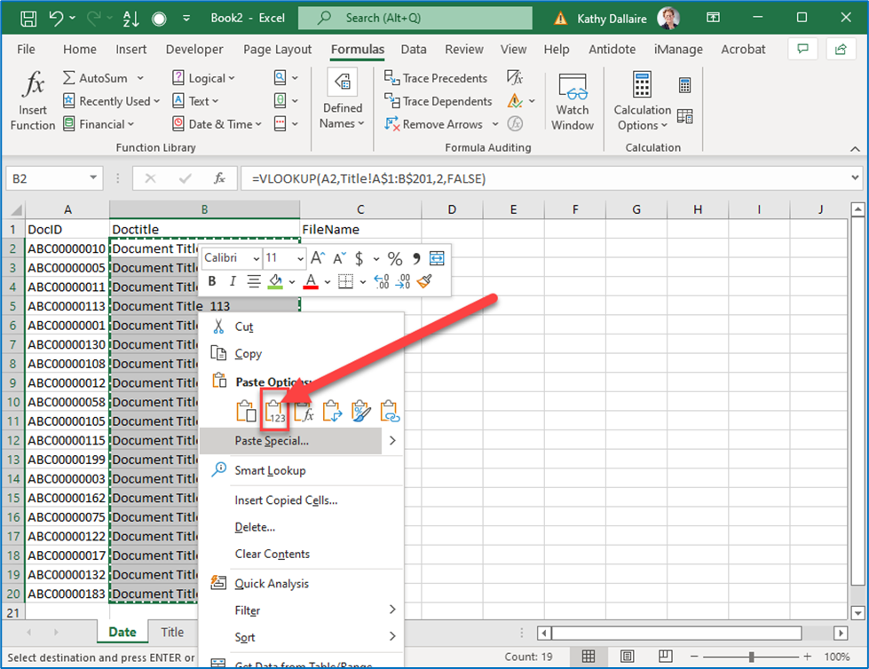
Right-click again and select paste text values:
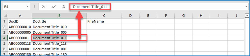
Notice that the formula bar now contains the text in the cell and not the original formula:
The same steps can now be used to search for the FileName values for column C from the third sheet in the spreadsheet.
While the VLOOKUP formula is very useful, it does have some limitations:
- the common identifier (DocID) must be located in the leftmost column
- the value that is being searched for must be to the right of the common document identifier.
Using the Concatenate or TEXTJOIN formulas to combine values into one cell
Both the CONCATENATE and TEXTJOIN formulas are used to combine the values in one or more cells, with or without additional text as a prefix, suffix or delimiter. Where the TEXTJOIN formula differs is that it allows you to skip cells were there are no values.
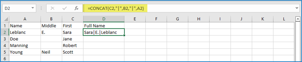
For example, where we want to combine the values for first name, middle name and last name from individual cells into one cell in a specific order, we can use the CONCATENATE formula.
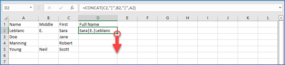
In the cell where we want the final combined value, start typing =concat and click on the formula button : 

Build the formula adding each argument in the order of the desired final result, separated by a space between quotes. (For the sake of this demonstration, the “|” symbol has been substituted for the space)
Click on the corner fill handle of the cell (or double-click on it) to copy the formula for the entire row:
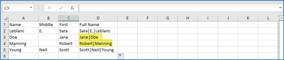
In this case, where there was no value in the Middle Name column, the concatenate formula still placed two delimiters with no value in between:
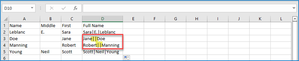
Using the TEXTJOIN formula solves this issue by automatically ignoring empty cells.
The TEXTJOIN formula uses the following arguments:
TEXTJOIN(delimiter, ignore_empty, text1, text2…)
delimiter What will separate each value, such as a space, a comma, etc. The delimiter is indicated between quotes ex: “ “ for a space.
ignore_empty By default, TextJoin ignores empty cells, so this argument can be left empty.
text1 Identify each cell to be combined, separated by a comma.
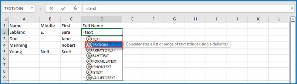
In the cell designated for the combined value, start typing =textjoin and click on the formula button : 
Build the formula adding arguments in the order of the desired final result separated by a space between quotes. (For the sake of this demonstration, the “|” symbol been substituted for the space).
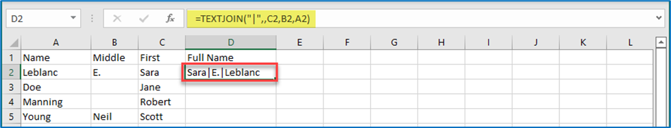
Click on the corner fill handle of the cell (or double-click on it) to copy the formula for the entire row:

In this case, where there was no value in the Middle Name column, the TEXTJOIN formula appropriately added only one required delimiter between the first and last name:
Please see the section on Hard-Coding Results to ensure the results are useable.
#LitigationSupportoreDiscovery#PracticeManagementandPracticeSupport#ProfessionalDevelopment#Firm